41 how to show data labels as percentage in excel
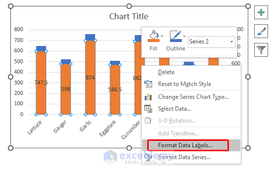
› how-to-format-chart-axisHow to Format Chart Axis to Percentage in Excel ... Jul 28, 2021 · By default, the Decimal places will be of 2 digits in the percentage representation. You can change it accordingly. In our case, we made it 0 decimal places. 5. Close the Format Axis dialog box. And finally, the chart has data in the form of percentage representation on the Y-axis. How to Show Percentage in Bar Chart in Excel (3 Handy Methods) - ExcelDemy Thirdly, go to Chart Element > Data Labels. Next, double-click on the label, following, type an Equal ( =) sign on the Formula Bar, and select the percentage value for that bar. In this case, we chose the C13 cell. In a similar fashion, repeat the process for the other values and finally, the results should look like the following.
Format numbers as percentages - support.microsoft.com Display numbers as percentages To quickly apply percentage formatting to selected cells, click Percent Style in the Number group on the Home tab, or press Ctrl+Shift+%. If you want more control over the format, or you want to change other aspects of formatting for your selection, you can follow these steps.
How to show data labels as percentage in excel
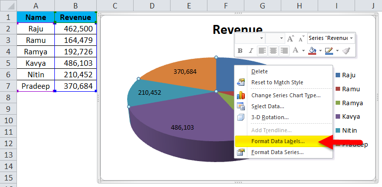
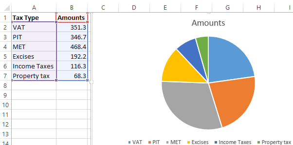
Excel Charts: How To Show Percentages in Stacked Charts (in ... - YouTube Download the workbook here: the full Excel Dashboard course here: h... Data label in the graph not showing percentage option. only value ... Data label in the graph not showing percentage option. only value coming Team, Normally when you put a data label onto a graph, it gives you the option to insert values as numbers or percentages. In the current graph, which I am developing, the percentage option not showing. Enclosed is the screenshot. › excel-pie-chart-percentageHow to Show Percentage in Excel Pie Chart (3 Ways) Sep 08, 2022 · We can open the Format Data Labels window in the following two ways. 2.1 Using Chart Elements. To active the Format Data Labels window, follow the simple steps below. Steps: Click on the pie chart to make it active. Now, click the Chart Elements button ( the Plus + sign at the top right corner of the pie chart). Click the Data Labels checkbox ...
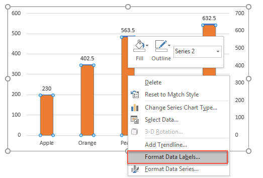
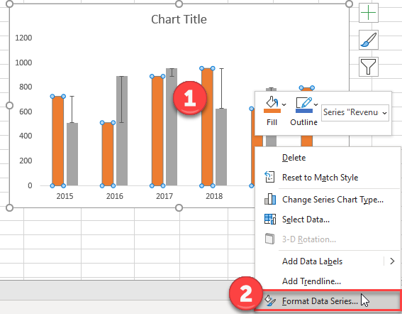
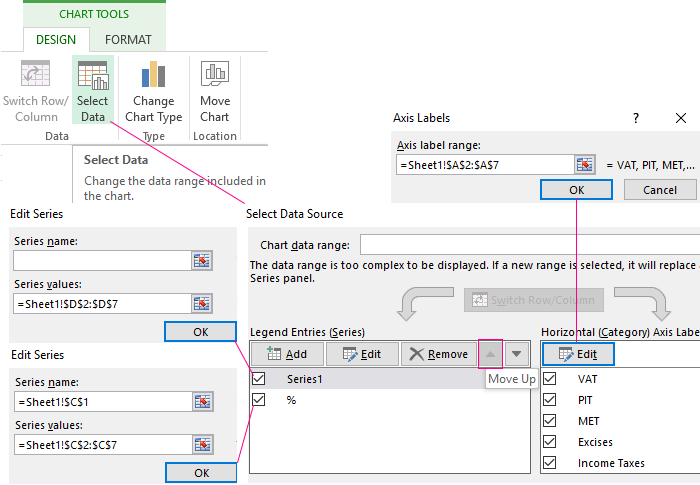
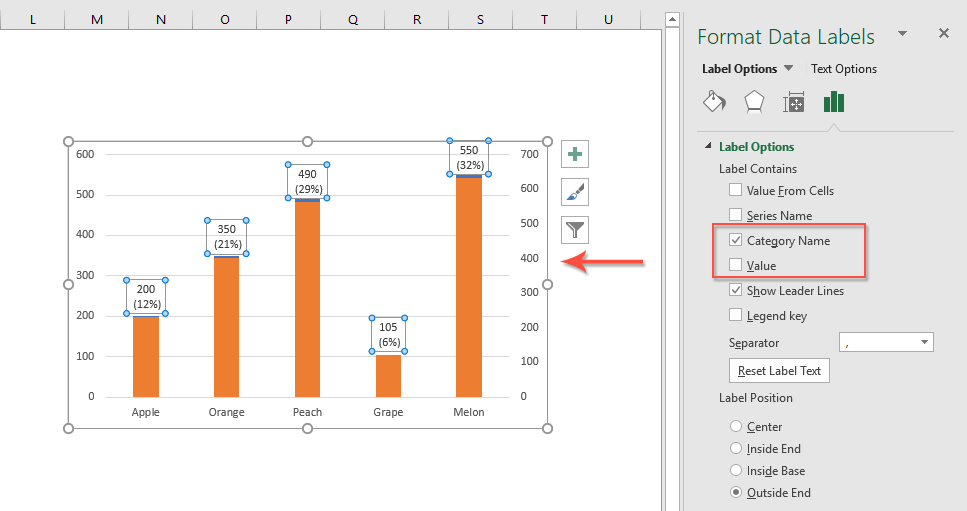
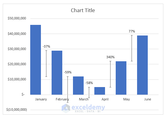
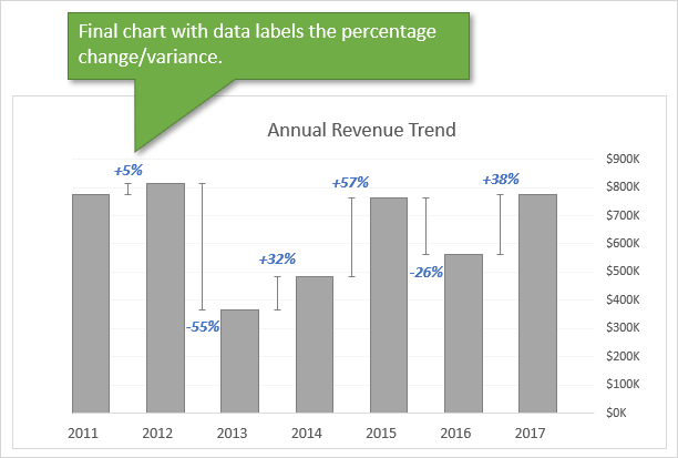
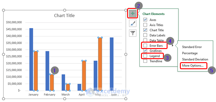
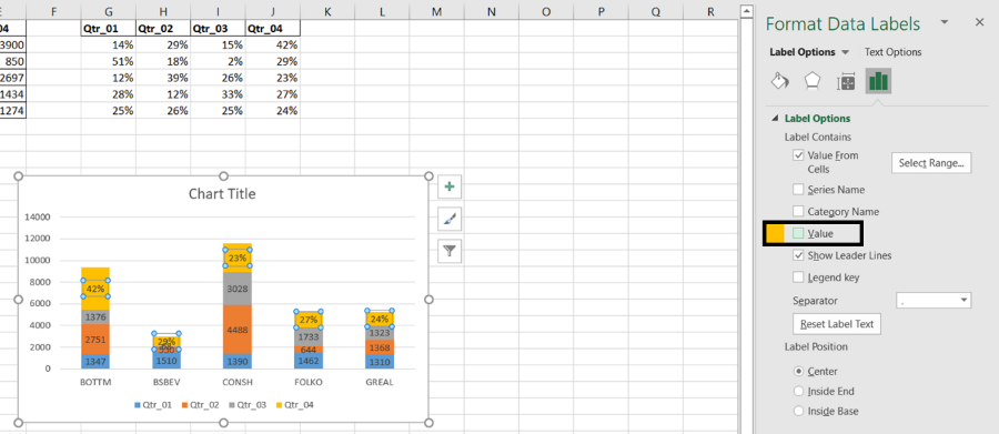
How to show data labels as percentage in excel. › en-us › microsoft-365Microsoft 365 Roadmap | Microsoft 365 You can create PivotTables in Excel that are connected to datasets stored in Power BI with a few clicks. Doing this allows you get the best of both PivotTables and Power BI. Calculate, summarize, and analyze your data with PivotTables from your secure Power BI datasets. More info. Feature ID: 63806; Added to Roadmap: 05/21/2020; Last Modified ... How to Show Percentage and Value in Excel Pie Chart - ExcelDemy From the Chart Element option, click on the Data Labels. These are the given results showing the data value in a pie chart. Right-click on the pie chart. Select the Format Data Labels command. Now click on the Value and Percentage options. Then click on the anyone of Label Positions. Here, we will click the Best Fit option. Change the format of data labels in a chart To get there, after adding your data labels, select the data label to format, and then click Chart Elements > Data Labels > More Options. To go to the appropriate area, click one of the four icons ( Fill & Line, Effects, Size & Properties ( Layout & Properties in Outlook or Word), or Label Options) shown here. › charts › column-chartColumn Chart That Displays Percentage Change or Variance Nov 01, 2018 · Select the Label Options sub menu in the Format Data Labels task pane. Click the Value from Cells checkbox. Select the range I5:I11 and press OK. Uncheck the Value and Show Leader Lines. The Label Position should be set to Outside End by default. For any negative variances, select each data label and change the position to Inside End.
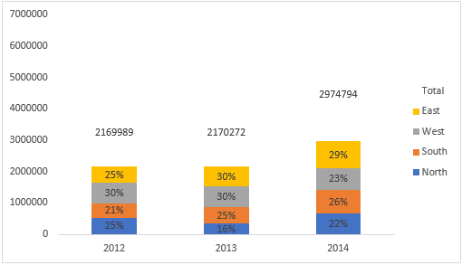
› how-to-show-percentages-inHow to Show Percentages in Stacked Column Chart in Excel? Dec 17, 2021 · Click Percent style (1) to convert your new table to show number with Percentage Symbol. Step 7: Select chart data labels and right-click, then choose “Format Data Labels”. Step 8: Check “Values From Cells”. Step 9: Above step popup an input box for the user to select a range of cells to display on the chart instead of default values. How to display percentage labels in pie chart in Excel - YouTube to display percentage labels in pie chart in Excel How to Show Number and Percentage in Excel Bar Chart From the right pane go to " Label Options " and check mark the " Value from cells ". A new window will appear asking for the range from your table. Henceforward, Choose the percentage values from the dataset and click OK. Change the " Separator " to " New line " from the drop-down list to get percentage values just below the numbers. How to show values in data labels of Excel Pareto Chart when chart is ... 2) Move Value data series to 2nd Axis 3) Change Value data series Fill from Automatic to No Fill 4) Change 2nd Vertical Axis Labels to None 5) Add Data Labels to Value data series Hope this helps. Steve=True D dendres New Member Joined Aug 1, 2015 Messages 14 Aug 3, 2015 #3 Hi Steve=True, Thank you for the help.
Data Labels in Excel Pivot Chart (Detailed Analysis) Next open Format Data Labels by pressing the More options in the Data Labels. Then on the side panel, click on the Value From Cells. Next, in the dialog box, Select D5:D11, and click OK. Right after clicking OK, you will notice that there are percentage signs showing on top of the columns. 4. Changing Appearance of Pivot Chart Labels How to show data label in "percentage" instead of - Microsoft Community Select Format Data Labels Select Number in the left column Select Percentage in the popup options In the Format code field set the number of decimal places required and click Add. (Or if the table data in in percentage format then you can select Link to source.) Click OK Regards, OssieMac Report abuse 8 people found this reply helpful · How to Display Percentage in an Excel Graph (3 Methods) Select Chart on the Format Data Labels dialog box. Uncheck the Value option. Check the Value From Cells option. Then you have to select cell ranges to extract percentage values. For this purpose, create a column called Percentage using the following formula: =E5/C5 The Final Graph with Percentage Change Add or remove data labels in a chart - support.microsoft.com Click Label Options and under Label Contains, select the Values From Cells checkbox. When the Data Label Range dialog box appears, go back to the spreadsheet and select the range for which you want the cell values to display as data labels. When you do that, the selected range will appear in the Data Label Range dialog box. Then click OK.
How to create a chart with both percentage and value in Excel?
change data label to percentage - Power BI 06-08-2020 11:22 AM. Hi @MARCreading. pick your column in the Right pane, go to Column tools Ribbon and press Percentage button. do not hesitate to give a kudo to useful posts and mark solutions as solution. LinkedIn. View solution in original post. Message 2 of 7.
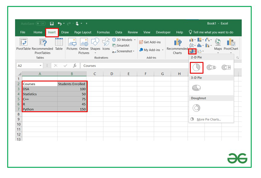
Pie Chart in Excel | How to Create Pie Chart | Step-by-Step ...
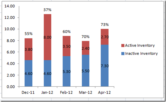
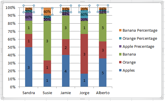
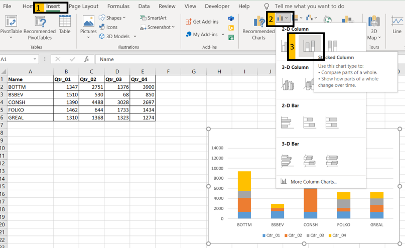
How to Add Percentages to Excel Bar Chart - Excel Tutorial We will select range A1:C8 and go to Insert >> Charts >> 2-D Column >> Stacked Column: Once we do this we will click on our created Chart, then go to Chart Design >> Add Chart Element >> Data Labels >> Inside Base: To lose the colors that we have on points percentage and to lose it in the title we will simply click anywhere on the small orange ...

Data Labels in Power BI - SPGuides
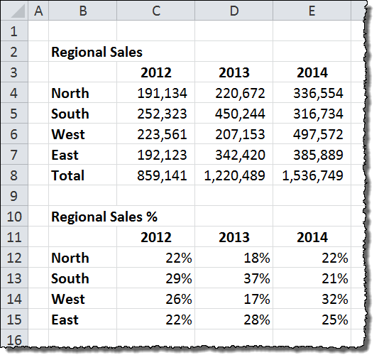
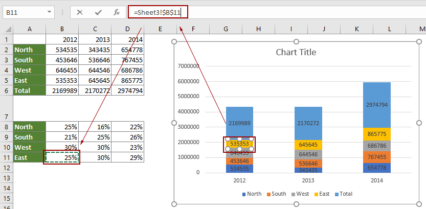
Stacked bar charts showing percentages (excel) - Microsoft Community What you have to do is - select the data range of your raw data and plot the stacked Column Chart and then add data labels. When you add data labels, Excel will add the numbers as data labels. You then have to manually change each label and set a link to the respective % cell in the percentage data range.

Microsoft Excel Tutorials: Add Data Labels to a Pie Chart
Excel data doesn't retain formatting in mail merge - Office Select File > Options. On the Advanced tab, go to the General section. Select the Confirm file format conversion on open check box, and then select OK. On the Mailings tab, select Start Mail Merge, and then select Step By Step Mail Merge Wizard. In the Mail Merge task pane, select the type of document that you want to work on, and then select Next.
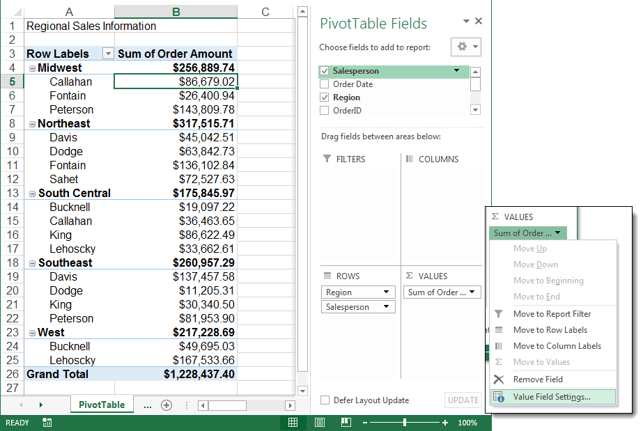
Pivot Table: Percentage of Total Calculations in Excel ...
How to Put Count and Percentage in One Cell in Excel? So in this article, we will learn how to display count and percentage in the same cell with the help of an example. In the below, sample data, have given sales data in $ and market share in Percentages. We need to add a column to show both Sales $ (Share %) in a cell as in (Img2). Sample Data:
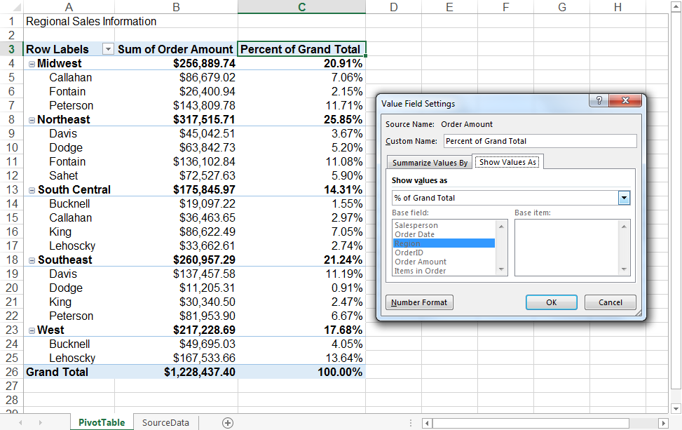
Pivot Table: Percentage of Total Calculations in Excel ...
Display the percentage data labels on the active chart. - YouTube Display the percentage data labels on the active chart.Want more? Then download our TEST4U demo from TEST4U provides an innovat...

Best Excel Tutorial - Chart with number and percentage
› excel-pie-chart-percentageHow to Show Percentage in Excel Pie Chart (3 Ways) Sep 08, 2022 · We can open the Format Data Labels window in the following two ways. 2.1 Using Chart Elements. To active the Format Data Labels window, follow the simple steps below. Steps: Click on the pie chart to make it active. Now, click the Chart Elements button ( the Plus + sign at the top right corner of the pie chart). Click the Data Labels checkbox ...
Percentage Change Chart – Excel – Automate Excel
Data label in the graph not showing percentage option. only value ... Data label in the graph not showing percentage option. only value coming Team, Normally when you put a data label onto a graph, it gives you the option to insert values as numbers or percentages. In the current graph, which I am developing, the percentage option not showing. Enclosed is the screenshot.
Percent charts in Excel: creation instruction
Excel Charts: How To Show Percentages in Stacked Charts (in ... - YouTube Download the workbook here: the full Excel Dashboard course here: h...

Choosing a Chart Type
Percent charts in Excel: creation instruction
How to show the percentage on stacked colum/bar chart in ...
How-to Put Percentage Labels on Top of a Stacked Column Chart ...

How to Show Pie Chart Data Labels in Percentage in Excel

How to create a chart with both percentage and value in Excel?
How to show percentages in stacked column chart in Excel?
How to Show Number and Percentage in Excel Bar Chart - ExcelDemy
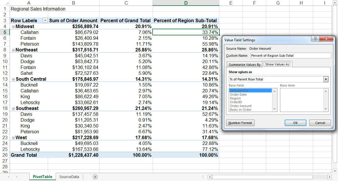
Pivot Table: Percentage of Total Calculations in Excel ...

Excel: Clustered Column Chart with Percent of Month ...

How to Add Data Labels to your Excel Chart in Excel 2013

Format Number Options for Chart Data Labels in PowerPoint ...

Count and Percentage in a Column Chart
How to create a chart with both percentage and value in Excel?

Excel: Clustered Column Chart with Percent of Month ...
How to Display Percentage in an Excel Graph (3 Methods ...

Is there a way to add data labels as percentages on the ...
How to Show Percentage in Pie Chart in Excel? - GeeksforGeeks

Add or remove data labels in a chart

Creating Pie Chart and Adding/Formatting Data Labels (Excel)
How to Show Percentages in Stacked Bar and Column Charts in Excel

Change the format of data labels in a chart

How to show percentages on three different charts in Excel ...
How to show percentages in stacked column chart in Excel?

Change the format of data labels in a chart
Column Chart That Displays Percentage Change or Variance ...
charts - Showing percentages above bars on Excel column graph ...
Friday Challenge Answer - Create a Percentage (%) and Value ...
How to Display Percentage in an Excel Graph (3 Methods ...
How to Show Percentages in Stacked Column Chart in Excel ...

How to Make Pie Chart with Labels both Inside and Outside ...
How to Show Percentages in Stacked Column Chart in Excel ...
Post a Comment for "41 how to show data labels as percentage in excel"