41 how to customize data labels in excel
How to add data labels from different column in an Excel chart? Right click the data series, and select Format Data Labels from the context menu. 3. In the Format Data Labels pane, under Label Options tab, check the Value From Cells option, select the specified column in the popping out dialog, and click the OK button. Now the cell values are added before original data labels in bulk. 4. How to Print Labels From Excel - Lifewire Choose Start Mail Merge > Labels . Choose the brand in the Label Vendors box and then choose the product number, which is listed on the label package. You can also select New Label if you want to enter custom label dimensions. Click OK when you are ready to proceed. Connect the Worksheet to the Labels
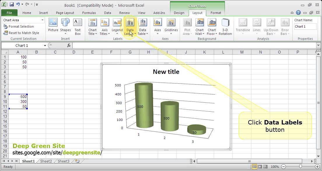
How to Change Excel Chart Data Labels to Custom Values? You can change data labels and point them to different cells using this little trick. First add data labels to the chart (Layout Ribbon > Data Labels) Define the new data label values in a bunch of cells, like this: Now, click on any data label. This will select "all" data labels. Now click once again.
How to customize data labels in excel
Custom data labels in a chart - Get Digital Help Press with right mouse button on on any data series displayed in the chart. Press with mouse on "Add Data Labels". Press with mouse on Add Data Labels". Double press with left mouse button on any data label to expand the "Format Data Series" pane. Enable checkbox "Value from cells". Format Data Labels in Excel- Instructions - TeachUcomp, Inc. To do this, click the "Format" tab within the "Chart Tools" contextual tab in the Ribbon. Then select the data labels to format from the "Chart Elements" drop-down in the "Current Selection" button group. Then click the "Format Selection" button that appears below the drop-down menu in the same area. How to I rotate data labels on a column chart so that they are ... To change the text direction, first of all, please double click on the data label and make sure the data are selected (with a box surrounded like following image). Then on your right panel, the Format Data Labels panel should be opened. Go to Text Options > Text Box > Text direction > Rotate
How to customize data labels in excel. Excel tutorial: How to customize axis labels Instead you'll need to open up the Select Data window. Here you'll see the horizontal axis labels listed on the right. Click the edit button to access the label range. It's not obvious, but you can type arbitrary labels separated with commas in this field. So I can just enter A through F. When I click OK, the chart is updated. How to Create Mailing Labels in Word from an Excel List Select the first label, switch to the "Mailings" tab, and then click "Address Block." In the "Insert Address Block" window that appears, click the "Match Fields" button. The "Match Fields" window will appear. In the "Required for Address Block" group, make sure each setting matches the column in your workbook. How Do I Create Avery Labels From Excel? - Ink Saver Arrange the fields: Next, arrange the columns and rows in the order they appear in your label. This step is optional but highly recommended if your designs look neat. For this, just double click or drag and drop them in the text box on your right. Don't forget to add commas and spaces to separate fields Add a DATA LABEL to ONE POINT on a chart in Excel All the data points will be highlighted. Click again on the single point that you want to add a data label to. Right-click and select ' Add data label '. This is the key step! Right-click again on the data point itself (not the label) and select ' Format data label '. You can now configure the label as required — select the content of ...
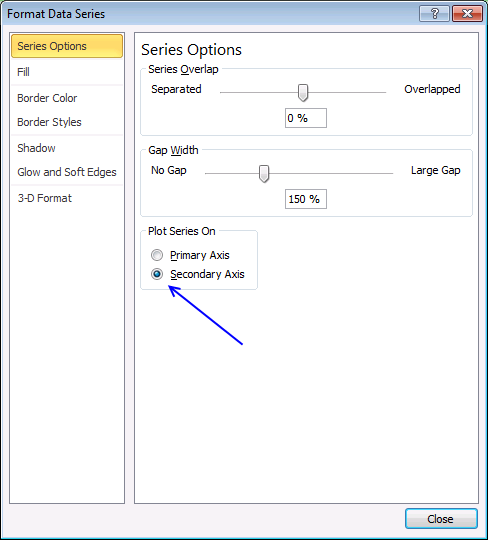
Add or remove data labels in a chart - support.microsoft.com Click Label Options and under Label Contains, pick the options you want. Use cell values as data labels You can use cell values as data labels for your chart. Right-click the data series or data label to display more data for, and then click Format Data Labels. Click Label Options and under Label Contains, select the Values From Cells checkbox. Custom Y-Axis Labels in Excel - PolicyViz 1. Select that column and change it to a scatterplot. 2. Select the point, right-click to Format Data Series and plot the series on the Secondary Axis. 3. Show the Secondary Horizontal axis by going to the Axes menu under the Chart Layout button in the ribbon. (Notice how the point moves over when you do so.) 4. Add / Move Data Labels in Charts - Excel & Google Sheets Click on the graph Select + Sign in the top right of the graph Check Data Labels Change Position of Data Labels Click on the arrow next to Data Labels to change the position of where the labels are in relation to the bar chart Final Graph with Data Labels Using the CONCAT function to create custom data labels for an Excel ... Use the chart skittle (the "+" sign to the right of the chart) to select Data Labels and select More Options to display the Data Labels task pane. Check the Value From Cells checkbox and select the cells containing the custom labels, cells C5 to C16 in this example. It is important to select the entire range because the label can move based ...
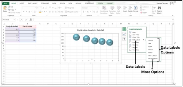
Add Custom Labels to x-y Scatter plot in Excel Step 1: Select the Data, INSERT -> Recommended Charts -> Scatter chart (3 rd chart will be scatter chart) Let the plotted scatter chart be. Step 2: Click the + symbol and add data labels by clicking it as shown below. Step 3: Now we need to add the flavor names to the label. Now right click on the label and click format data labels. How to Create Labels in Word from an Excel Spreadsheet Select Browse in the pane on the right. Choose a folder to save your spreadsheet in, enter a name for your spreadsheet in the File name field, and select Save at the bottom of the window. Close the Excel window. Your Excel spreadsheet is now ready. 2. Configure Labels in Word. How to Customize Your Excel Pivot Chart Data Labels To add data labels, just select the command that corresponds to the location you want. To remove the labels, select the None command. If you want to specify what Excel should use for the data label, choose the More Data Labels Options command from the Data Labels menu. Excel displays the Format Data Labels pane. how to add data labels into Excel graphs - storytelling with data There are a few different techniques we could use to create labels that look like this. Option 1: The "brute force" technique. The data labels for the two lines are not, technically, "data labels" at all. A text box was added to this graph, and then the numbers and category labels were simply typed in manually.
Add or Remove Data Labels in excel - YouTube
How To Create Labels In Excel • Visual Inc Make Row Labels In Excel 2007 Freeze For Easier Reading from . Starting document near the bottom. Click a data label one time to select all data labels in a data series or two times to select just one data label that you want to delete, and then press delete. Click finish & merge in the finish group on the mailings tab.
Custom data labels in a chart | Get Digital Help - Microsoft Excel resource
How to add and customize chart data labels - Get Digital Help Double press with left mouse button on with left mouse button on a data label series to open the settings pane. Go to tab "Label Options" see image to the right. This setting allows you to change the number formatting of the data labels. The image below shows numbers formatted as dates. Fill
Using Excel 2010 - Add Data Labels - YouTube
How to Create Mailing Labels in Excel | Excelchat In this tutorial, we will learn how to use a mail merge in making labels from Excel data, set up a Word document, create custom labels and print labels easily. Figure 1 - How to Create Mailing Labels in Excel. Step 1 - Prepare Address list for making labels in Excel. First, we will enter the headings for our list in the manner as seen below.
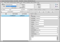
Free Employee Phone Directory 2 database template for Organizer Deluxe and Pro users, windows
How to Use Cell Values for Excel Chart Labels Select the chart, choose the "Chart Elements" option, click the "Data Labels" arrow, and then "More Options.". Uncheck the "Value" box and check the "Value From Cells" box. Select cells C2:C6 to use for the data label range and then click the "OK" button. The values from these cells are now used for the chart data labels.
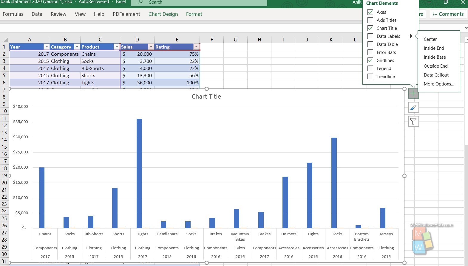
How To Show Or Hide Data Labels On MS Excel? | My Windows Hub
Custom Chart Data Labels In Excel With Formulas Follow the steps below to create the custom data labels. Select the chart label you want to change. In the formula-bar hit = (equals), select the cell reference containing your chart label's data. In this case, the first label is in cell E2. Finally, repeat for all your chart laebls.
:max_bytes(150000):strip_icc()/PreparetheWorksheet2-5a5a9b290c1a82003713146b.jpg)
How to Make Labels from Excel
Change the format of data labels in a chart To get there, after adding your data labels, select the data label to format, and then click Chart Elements > Data Labels > More Options. To go to the appropriate area, click one of the four icons ( Fill & Line, Effects, Size & Properties ( Layout & Properties in Outlook or Word), or Label Options) shown here.
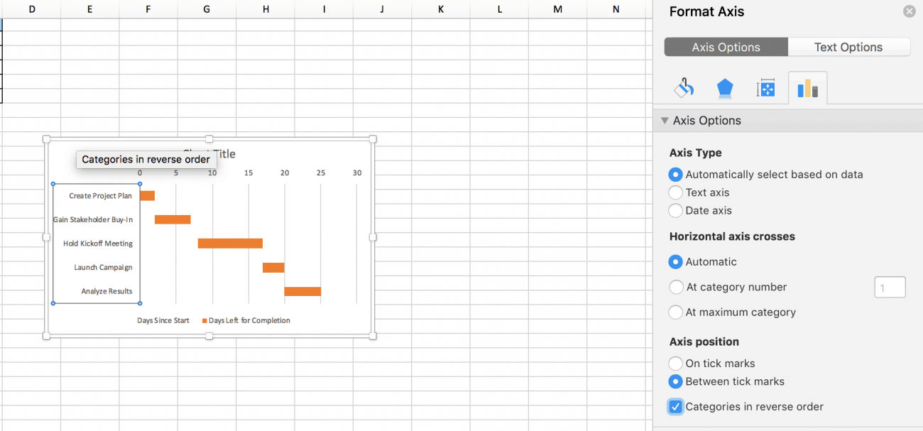
Free Gantt Charts in Excel: Templates, Tutorial & Video | Smartsheet
How to create label cards in Excel - Ablebits If you choose to get more than one column with the results, you can also divide them By empty column. Save original headers and formatting: Tick the Add header checkbox to display all column headers as labels next to the values in your cards. It is possible to keep the format of your original data by ticking the Preserve formatting checkbox. Note.
Advanced Excel - более богатые метки данных - CoderLessons.com
How to create Custom Data Labels in Excel Charts Two ways to do it. Click on the Plus sign next to the chart and choose the Data Labels option. We do NOT want the data to be shown. To customize it, click on the arrow next to Data Labels and choose More Options … Unselect the Value option and select the Value from Cells option. Choose the third column (without the heading) as the range.

To Do List Template Excel ~ Addictionary
Excel tutorial: How to use data labels Generally, the easiest way to show data labels to use the chart elements menu. When you check the box, you'll see data labels appear in the chart. If you have more than one data series, you can select a series first, then turn on data labels for that series only. You can even select a single bar, and show just one data label.

How to Create Progress Charts (Bar and Circle) in Excel - Automate Excel
Custom Data Labels with Colors and Symbols in Excel Charts - [How To] To apply custom format on data labels inside charts via custom number formatting, the data labels must be based on values. You have several options like series name, value from cells, category name. But it has to be values otherwise colors won't appear. Symbols issue is quite beyond me.

Excel Course: Inserting Graphs
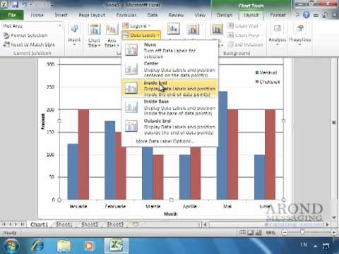
How to add or move data labels in Excel chart? - ExtendOffice 2. Then click the Chart Elements, and check Data Labels, then you can click the arrow to choose an option about the data labels in the sub menu. See screenshot: In Excel 2010 or 2007. 1. click on the chart to show the Layout tab in the Chart Tools group. See screenshot: 2. Then click Data Labels, and select one type of data labels as you need ...

Printable Church Directory Template: 6+ Free Documents in Excel, Word & PDF
How to I rotate data labels on a column chart so that they are ... To change the text direction, first of all, please double click on the data label and make sure the data are selected (with a box surrounded like following image). Then on your right panel, the Format Data Labels panel should be opened. Go to Text Options > Text Box > Text direction > Rotate
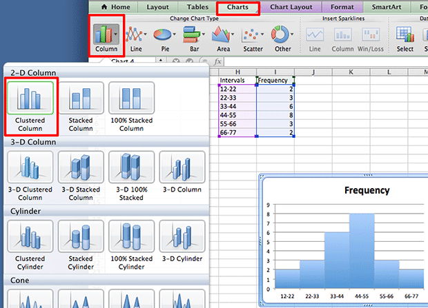
Create a Histogram Graph in Excel
Format Data Labels in Excel- Instructions - TeachUcomp, Inc. To do this, click the "Format" tab within the "Chart Tools" contextual tab in the Ribbon. Then select the data labels to format from the "Chart Elements" drop-down in the "Current Selection" button group. Then click the "Format Selection" button that appears below the drop-down menu in the same area.
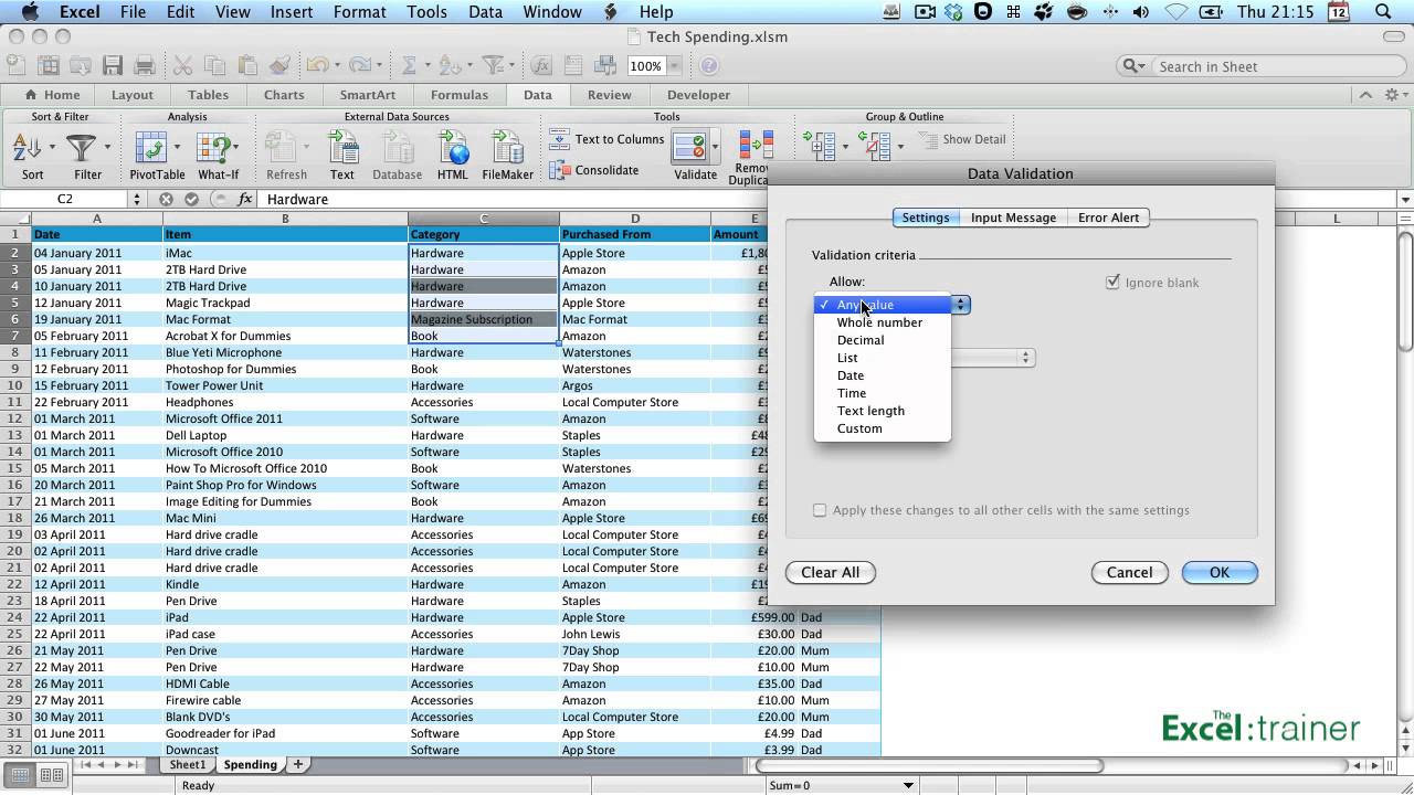
Excel : Data Validation & Drop Down Lists - YouTube
Custom data labels in a chart - Get Digital Help Press with right mouse button on on any data series displayed in the chart. Press with mouse on "Add Data Labels". Press with mouse on Add Data Labels". Double press with left mouse button on any data label to expand the "Format Data Series" pane. Enable checkbox "Value from cells".

Format Data Labels in Excel- Instructions | Microsoft excel, Microsoft, Bar chart

31 What Is Data Label In Excel - Labels Database 2020
Free Inventory Template + How to Track and Count Physical Inventory
MS Excel 2010 / How to remove data labels from the chart - YouTube
Post a Comment for "41 how to customize data labels in excel"