38 excel chart labels from cells
How to add text labels on Excel scatter chart axis In addition, I would like to add custom labels on Excel scatter chart x-axis with each person's name. Stepps to add text labels on Excel scatter chart axis. 1. ... Add custom data labels from the column "X axis labels". Use "Values from Cells" like in this other post and remove values related to the actual dummy series. Change the ... How to add data labels in excel to graph or chart (Step-by-Step) Add data labels to a chart. 1. Select a data series or a graph. After picking the series, click the data point you want to label. 2. Click Add Chart Element Chart Elements button > Data Labels in the upper right corner, close to the chart. 3. Click the arrow and select an option to modify the location. 4.
Add or remove data labels in a chart - Microsoft Support

Excel chart labels from cells
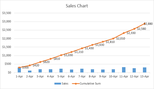
Chart.ApplyDataLabels method (Excel) | Microsoft Docs The type of data label to apply. True to show the legend key next to the point. The default value is False. True if the object automatically generates appropriate text based on content. For the Chart and Series objects, True if the series has leader lines. Pass a Boolean value to enable or disable the series name for the data label. Custom Chart Data Labels In Excel With Formulas Excel Chart Data Labels Using Formulas. In Column D I added is the difference between April 2016 sales and the previous months sales, whereas in Column E is where I have my custom labels that appear on my chart. The Formula is D is a standard % difference formula, taking the difference between the two numbers and dividing it by the original number. DataLabel object (Excel) | Microsoft Docs Use the DataLabel property of the Point object to return the DataLabel object for a single point. The following example turns on the data label for the second point in series one on the chart sheet named Chart1, and sets the data label text to Saturday. On a trendline, the DataLabel property returns the text shown with the trendline.
Excel chart labels from cells. excel - Adding labels to line chart with VBA - Stack Overflow The chart that is printed looks something like this. I'm trying to figure out how to add labels to arbitrary points to the chart. Two labels to be specific. One is at the minimum value. And one is the value at any arbitrary point on x-axis. Both x-values are known and will be taken as inputs from two cells on the sheet. Something like this. How do you label data points in Excel? - profitclaims.com 1. Right click the data series in the chart, and select Add Data Labels > Add Data Labels from the context menu to add data labels. 2. Click any data label to select all data labels, and then click the specified data label to select it only in the chart. 3. Extract from cells into labels [SOLVED] - excelforum.com Re: Extract from cells into labels. I would use the WORD Mail Merge function with output on required labels with Excel file being the data source. If that takes care of your original question, please select Thread Tools from the menu link above and mark this thread as SOLVED. Register To Reply. 04-26-2022, 09:37 AM #7. Conditional Data Labels in Charts - Microsoft Tech Community Its dynamic and will change between time labels. My issue is that sometimes the data contains 0 values that aren't true zeros. Ie. They represent data that was suppressed. In the chart, I want to make mention of them by having a data label for just those points with an "x" to represent the suppression. Ie. I would like a way to have the x data l.
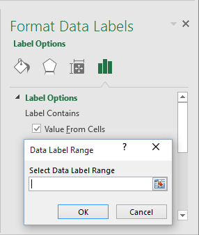
Pivot chart label - Microsoft Tech Community HI, I want to create a pivot chart but I want to use a different column for the label which is made of the concatenate value of 2 columns. Can this be done?. By using Format Data Labels and Value From Cells (select Range) is not working as this option will be giving the value of the data in order and not taking into account the different ... How to Add Labels to Scatterplot Points in Excel - Statology Step 3: Add Labels to Points. Next, click anywhere on the chart until a green plus (+) sign appears in the top right corner. Then click Data Labels, then click More Options…. In the Format Data Labels window that appears on the right of the screen, uncheck the box next to Y Value and check the box next to Value From Cells. Dynamic Chart Title by Linking and Reference to Cell in Excel Linking Cell to make Dynamic Chart Title - Step 1: Select a Chart Title. Identify the chart to link a cell reference to the chart title. The following screen-shot will show you example chart title is selected. Dynamic chart title- Cell linking to chart title. Here you can clearly observe that there is no formula is associated to chart title. excel - Adding Data Label To Chart Based On X Values - Stack Overflow Here's my setup. Categories, including maybe "Red" in column A, Values in column B, and chart labels in column C. In cell C2 I'm using a formula like this: =IF (A2="Red","Label Text Here","") so there is only text in that column if the X value is "Red". My chart plots columns A and B of the data range. I added data labels, then formatted the ...
How to Print Labels from Excel - Lifewire Select Mailings > Write & Insert Fields > Update Labels . Once you have the Excel spreadsheet and the Word document set up, you can merge the information and print your labels. Click Finish & Merge in the Finish group on the Mailings tab. Click Edit Individual Documents to preview how your printed labels will appear. Select All > OK . How do you mail merge labels from Excel? - Vivu.tv How to Turn Excel Cells Into Mailing Labels. 1. Open Excel 2010 and click the 'File' tab. Click 'Open.'. Browse the files and locate a workbook. Click the workbook and the 'Open' button. The workbook will open. 2. Review the workbook and make sure the data that will be used in the mailing labels contains column headers. Excel column labels turn white and gridlines disappear when scrolling The column labels and row labels turn white when scrolling in excel. Grind lines also disappear when scrolling and only appear after manually unchecking and then checking the show gridlines button. I have tried everything I found online so far: I updated the graphics driver, I reinstalled office, I tried to " Disable hardware graphics ... How to Find, Highlight, and Label a Data Point in Excel Scatter Plot? By default, the data labels are the y-coordinates. Step 3: Right-click on any of the data labels. A drop-down appears. Click on the Format Data Labels… option. Step 4: Format Data Labels dialogue box appears. Under the Label Options, check the box Value from Cells . Step 5: Data Label Range dialogue-box appears.
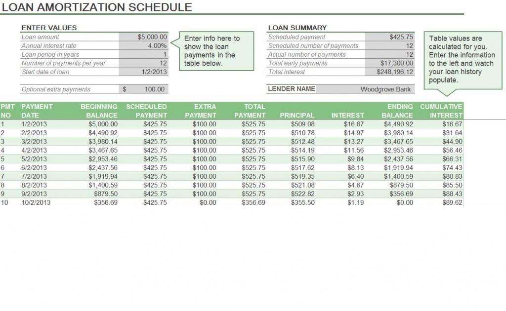
Amortization Formula Excel | Excel Amortization Formula
Excel: How to Create a Bubble Chart with Labels - Statology Step 3: Add Labels. To add labels to the bubble chart, click anywhere on the chart and then click the green plus "+" sign in the top right corner. Then click the arrow next to Data Labels and then click More Options in the dropdown menu: In the panel that appears on the right side of the screen, check the box next to Value From Cells within ...

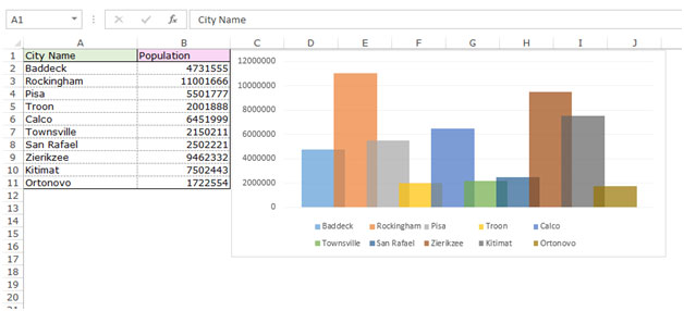
How to Use Cell Values for Excel Chart Labels
Scatter Chart Format Labels from Multiple Cells [SOLVED] I am creating a scatter chart with data labels pulled from cells. However, where one data point has a label from multiple cells, the text of the labels are appearing on top of one another, causing overlap. I created a small example attached. In the image you can see that because Dirk and Howard have the same age and weight, the data point for ...

35 Label Cells In Excel - Label Design Ideas 2020
Where labels are aligned in cells? - TimesMojo Aligning Data Label Text Select the series of data labels to align all the text in the series. Select an individual data label to align its text. Choose the Format Data Labels option and choose the Alignment tab, shown below. Click Apply to see your changes or OK to acceptRead More →
Displaying Numbers in Thousands in a Chart in Microsoft Excel
Data Labels in Excel Pivot Chart (Detailed Analysis) Add a Pivot Chart from the PivotTable Analyze tab. Then press on the Plus right next to the Chart. Next open Format Data Labels by pressing the More options in the Data Labels. Then on the side panel, click on the Value From Cells. Next, in the dialog box, Select D5:D11, and click OK.
Creating a chart with dynamic labels - Microsoft Excel 2016
How to Change Font Size of Data Labels in Excel - ExcelDemy Steps: Initially, select the whole data and go to the Insert tab. After that, click on the 2-D Pie. After getting the proper pie chart, select the whole chart and choose Data Labels from the Chart Elements. Then, select the data and go to the Home tab. Afterward, choose the proper font size according to your need.

Bubble Chart: How to create it in excel - DataWitzz
How do I change the labels on an Excel chart? - Foley for Senate How to Add Data Labels to an Excel 2010 Chart. Click anywhere on the chart that you want to modify. On the Chart Tools Layout tab, click the Data Labels button in the Labels group. Select where you want the data label to be placed. On the Chart Tools Layout tab, click Data Labels→More Data Label Options.
Creating a chart with dynamic labels - Microsoft Excel 2016
DataLabel object (Excel) | Microsoft Docs Use the DataLabel property of the Point object to return the DataLabel object for a single point. The following example turns on the data label for the second point in series one on the chart sheet named Chart1, and sets the data label text to Saturday. On a trendline, the DataLabel property returns the text shown with the trendline.
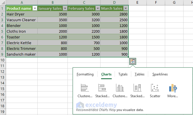
Excel Create A Chart From The Selected Range Of Cells - Chart Walls
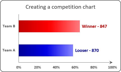
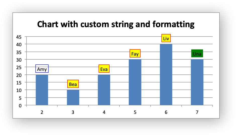
Custom Chart Data Labels In Excel With Formulas Excel Chart Data Labels Using Formulas. In Column D I added is the difference between April 2016 sales and the previous months sales, whereas in Column E is where I have my custom labels that appear on my chart. The Formula is D is a standard % difference formula, taking the difference between the two numbers and dividing it by the original number.
Example: Charts with Data Labels — XlsxWriter Documentation
Chart.ApplyDataLabels method (Excel) | Microsoft Docs The type of data label to apply. True to show the legend key next to the point. The default value is False. True if the object automatically generates appropriate text based on content. For the Chart and Series objects, True if the series has leader lines. Pass a Boolean value to enable or disable the series name for the data label.
Excel Cell Equals Tab Name
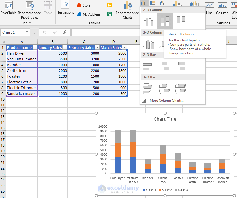
Excel Create A Chart From The Selected Range Of Cells - Chart Walls

Two top easiest ways to create a dynamic range in Excel chart
Chart with a Dual Category Axis - Peltier Tech Blog
Simple Excel
How to do a running total in Excel (Cumulative Sum formula)

How to Count Unique Values in Excel 2016? (with Pictures) - QueHow
How to Chart Cells From Two Different Worksheets in Microsoft Excel : Using MS Excel - YouTube
Post a Comment for "38 excel chart labels from cells"